The requirement of large thermal stability of the recording media
implies large energy barriers. Therefore, the next step is their
evaluation for the grains of the previous section. For this purpose we
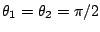
used the Lagrange multiplier method presented in Section 2.3.6. Fig. 3.33 shows the energy
barrier calculation for both model I and II as a function of the
(perpendicular) interfacial exchange. Initially, the system is
considered in the minimum that corresponds to all the moments aligned
and to the coordinates  in the energy landscapes
plotted in Figs. 3.34 and 3.35. Recall that
in the energy landscapes
plotted in Figs. 3.34 and 3.35. Recall that  is the average magnetization polar angle.
The final state will be the equivalent minimum but with the moments
pointing in the opposite direction, namely,
is the average magnetization polar angle.
The final state will be the equivalent minimum but with the moments
pointing in the opposite direction, namely,
 .
For small values of the interfacial exchange, there is an intermediate
minimum (see Fig. 3.34) and, therefore,
additional reversal modes and saddle points. In this situation
the soft grain can switch first with very low energy barrier and the
hard magnetic material will follow with a reduced energy barrier value.
However, the energy barrier corresponding to the inverse process,
namely, returning to the original minimum, is very small and the
probability of the inverse process to take place is high. Fig. 3.34 shows the effective energy landscape and
relevant configurations. The saddle points configurations are curled to
minimize the magnetostatic energy of the soft material.
For interfacial exchange energy higher than
.
For small values of the interfacial exchange, there is an intermediate
minimum (see Fig. 3.34) and, therefore,
additional reversal modes and saddle points. In this situation
the soft grain can switch first with very low energy barrier and the
hard magnetic material will follow with a reduced energy barrier value.
However, the energy barrier corresponding to the inverse process,
namely, returning to the original minimum, is very small and the
probability of the inverse process to take place is high. Fig. 3.34 shows the effective energy landscape and
relevant configurations. The saddle points configurations are curled to
minimize the magnetostatic energy of the soft material.
For interfacial exchange energy higher than  of
the bulk exchange in all cases, the energy barrier values saturate as a
function of
of
the bulk exchange in all cases, the energy barrier values saturate as a
function of  and
correspond to collective reversal. The collective modes are different
for the two models. In model I the thermal mode is almost coherent (see
Fig. 3.36(a)). The maximum energy
barrier value is determined by the quantity
and
correspond to collective reversal. The collective modes are different
for the two models. In model I the thermal mode is almost coherent (see
Fig. 3.36(a)). The maximum energy
barrier value is determined by the quantity
 . In the
model II, the
value of the energy barrier coincides with the domain
wall energy in the hard magnetic material as observed by D.Suess [Suess 05b] and the saddle point
is a domain wall centered in the hard material (see Fig. 3.36(b)).
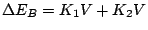
These differences can be appreciated in the effective energy Fig. 3.35. If the point
. In the
model II, the
value of the energy barrier coincides with the domain
wall energy in the hard magnetic material as observed by D.Suess [Suess 05b] and the saddle point
is a domain wall centered in the hard material (see Fig. 3.36(b)).
These differences can be appreciated in the effective energy Fig. 3.35. If the point
 is the saddle point, the energy
barrier corresponds to coherent rotation. For a non-homogeneous mode
the saddle point has to be elsewhere as in Fig. 3.35(b).
is the saddle point, the energy
barrier corresponds to coherent rotation. For a non-homogeneous mode
the saddle point has to be elsewhere as in Fig. 3.35(b).
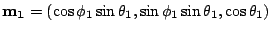
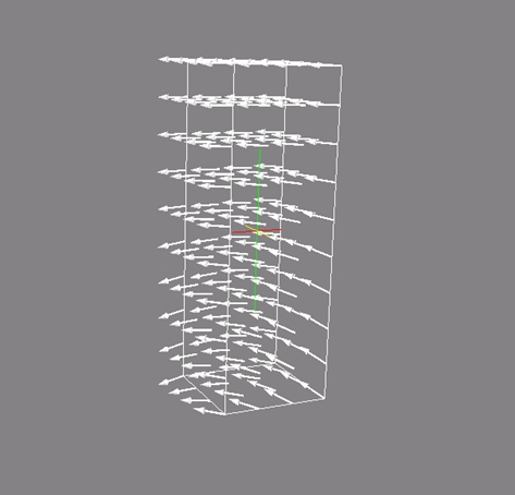
Figure:
Effective energy landscape and magnetic moment configurations in the
model I for  ,
,
 and
and  and corresponding
configuration for saddle points and minima.
and corresponding
configuration for saddle points and minima.
|
|
Figure:
Effective energy landscapes : (a) Model I
 , and
, and
 (b) Model
II ,
and
(b) Model
II ,
and  .
.
|
|
|
|
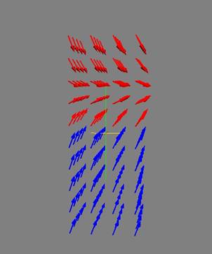
Figure 3.36:
Saddle point configuration for different mechanism: (a) Coherent
rotation (Model I) (b) Domain wall (Model II).
|
|
|
|
To get a better understanding of the energy barriers in a soft/hard
material, we can examine the case of model I for
, with a
model similar to that of Ref. [Victora 05a].
The
model
supposes
a macro-spin for each material. In such a model the energy is:
 |
(3.8) |
where 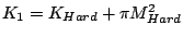 and
and
 are the
effective
anisotropy constants,
are the
effective
anisotropy constants,  is the number of atoms in the
surface,
is the number of atoms in the
surface,  is the volume of
each material
and finally
is the volume of
each material
and finally
 and
and
 are the
unit vector of the macrospin of each grain. To analyze the
problem, we have to consider the energy gradient and the Hessian
matrix. For large values of
there is only one energy barrier corresponding to the point
are the
unit vector of the macrospin of each grain. To analyze the
problem, we have to consider the energy gradient and the Hessian
matrix. For large values of
there is only one energy barrier corresponding to the point
 which value is
 . For
small interfacial exchange, there are additional barriers and saddle
points similar to the ones plotted in Fig. 3.34.
The
critical
exchange
for the crossover between the region is:
. For
small interfacial exchange, there are additional barriers and saddle
points similar to the ones plotted in Fig. 3.34.
The
critical
exchange
for the crossover between the region is:
 |
(3.9) |
In our system  .
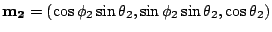
Finally, we can compare the analytical results with our simulations for
the same values of the constants. From Fig. 3.37, it is clear that there is a good
quantitative and qualitative agreement. These results indicate that the
two macro-spins is a good approximation for small interfacial exchange.
Nevertheless, this model is not valid for large exchange, where highly
nonhomogeneous modes are expected.
.
Finally, we can compare the analytical results with our simulations for
the same values of the constants. From Fig. 3.37, it is clear that there is a good
quantitative and qualitative agreement. These results indicate that the
two macro-spins is a good approximation for small interfacial exchange.
Nevertheless, this model is not valid for large exchange, where highly
nonhomogeneous modes are expected.
Figure:
(a) Comparison between the analytical model (solid lines) and numerical
calculations (symbols) for and
in model
I. (b) Energy contour plot from Eq. (3.8)
for  .
.
|
|
|
|
2008-04-04
![\includegraphics[width=0.9\textwidth]{Capitulo3/Graficas3/saddle}](img602.gif)
![\includegraphics[height=6cm]{Capitulo3/Graficas3/comparison}](img615.gif)
![\includegraphics[height=6cm]{Capitulo3/Graficas3/ebarrier}](img616.gif)
![\includegraphics[height=6cm]{Capitulo3/Graficas3/landscape.eps}](img603.gif)