Next: 2.2.2 Atomistic models in Up: 2.2 Linking different spatial Previous: 2.2 Linking different spatial Contents
Spin ![]() and orbital
and orbital ![]() moments, its coupling and the
exchange
interaction are pure quantum phenomena responsible for the
ferromagnetism. With simple quantum statistical models we can
explain some observed effects as the magnetocrystalline anisotropy
moments, its coupling and the
exchange
interaction are pure quantum phenomena responsible for the
ferromagnetism. With simple quantum statistical models we can
explain some observed effects as the magnetocrystalline anisotropy
![]() temperature dependence
exponent [Callen 66], where
temperature dependence
exponent [Callen 66], where
![]() is the order of the
spherical harmonics describing the angular
dependence of the local anisotropy, known as Callen-Callen or Akulov
law. Another example is the
is the order of the
spherical harmonics describing the angular
dependence of the local anisotropy, known as Callen-Callen or Akulov
law. Another example is the ![]() temperature
dependence of magnetization deviation from its
temperature
dependence of magnetization deviation from its ![]() value or Bloch law [Bloch 30]. However, analytical
models
are not able to treat complex systems and to extract the intrinsic
parameters of magnetic materials. In the mentioned above example of
the magnetic anisotropy temperature dependence the analytical
calculation is not able to provide the zero temperature value,
needed in order to complete the whole temperature dependence. First
principles numerical calculations are the tool needed to provide the
strength of the interactions and the structure of the material at
the atomic level. Unfortunately, the full Hamiltonian eigenvalue
problem is still only solvable in few cases and extra approximations
are needed. The first of them is the Born-Oppenheimer approximation
in which only the electronic degrees of freedom are taken into
account quantically and the nuclei move in the resulting ionic
potential. Another very useful approximation is to consider only
the outer electrons and to treat the inner electrons as
pseudopotential acting on the outer electrons. A powerful and amply
used tool is found in the density functional theory (DFT) which has its
origin in the
Hohenberg-Kohn Theorem that transforms the complex many-body problem
of interacting electrons and nuclei into a coupled set of
one-particle Kohn-Sham equations. The problem changes from a
eigenvalue problem to a variational problem, which is
computationally much more manageable. The energy becomes a
functional of the electronic density
value or Bloch law [Bloch 30]. However, analytical
models
are not able to treat complex systems and to extract the intrinsic
parameters of magnetic materials. In the mentioned above example of
the magnetic anisotropy temperature dependence the analytical
calculation is not able to provide the zero temperature value,
needed in order to complete the whole temperature dependence. First
principles numerical calculations are the tool needed to provide the
strength of the interactions and the structure of the material at
the atomic level. Unfortunately, the full Hamiltonian eigenvalue
problem is still only solvable in few cases and extra approximations
are needed. The first of them is the Born-Oppenheimer approximation
in which only the electronic degrees of freedom are taken into
account quantically and the nuclei move in the resulting ionic
potential. Another very useful approximation is to consider only
the outer electrons and to treat the inner electrons as
pseudopotential acting on the outer electrons. A powerful and amply
used tool is found in the density functional theory (DFT) which has its
origin in the
Hohenberg-Kohn Theorem that transforms the complex many-body problem
of interacting electrons and nuclei into a coupled set of
one-particle Kohn-Sham equations. The problem changes from a
eigenvalue problem to a variational problem, which is
computationally much more manageable. The energy becomes a
functional of the electronic density ![]() . The exact functional is
not known, because the exchange and correlation terms are not, and
additional approximation have to be invoked: Local Density
Approximation(LDA), General Gradient Approximation(GGA) , etc.
. The exact functional is
not known, because the exchange and correlation terms are not, and
additional approximation have to be invoked: Local Density
Approximation(LDA), General Gradient Approximation(GGA) , etc.
In the magnetic systems variations have to be included: our scheme
has to be spin aware (instead of LDA the local spin density(LSDA) is
used). The relativistic spin-orbit coupling has to be added to
the functional in order to calculate the magnetocrystalline
anisotropy. This term is very weak and can be considered as a
perturbation but provokes the need to change the representation from
![]() to the total angular
moment
to the total angular
moment ![]() because
because ![]() and
and ![]() are no
longer good quantum numbers.
are no
longer good quantum numbers.
An example of ab-initio calculations is the work on the magnetic
anisotropy of FePt ![]() [Mryasov 05], which is one of the
principle materials under investigation in this thesis. In what
follows, we will use the FePt parameters, estimated in this work.
The high anisotropy fct FePt
[Mryasov 05], which is one of the
principle materials under investigation in this thesis. In what
follows, we will use the FePt parameters, estimated in this work.
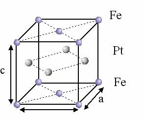
The high anisotropy fct FePt ![]() phase consists of alternated
atomic layers of Fe and Pt (see Fig. 2.2).
The
magntetocristallyne anisotropy is mainly due to the contribution
from the 5d element (Pt) having large spin-orbit coupling whereas
the 3d element (Fe) provides the large magnetic moment. The work
uses the constrained LSDA (CLSDA) method, which allows to treat
non-collinear magnetic order [Dederichs 84].
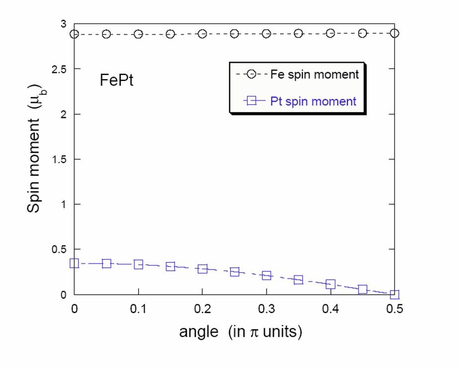
The Pt, normally
non-magnetic, has an induced non-localized magnetic moment (see
Fig. 2.3) proportional to the exchange
field from
the Fe moments. Treating the Pt moments as independent degrees of
freedom gives incorrect results (low
phase consists of alternated
atomic layers of Fe and Pt (see Fig. 2.2).
The
magntetocristallyne anisotropy is mainly due to the contribution
from the 5d element (Pt) having large spin-orbit coupling whereas
the 3d element (Fe) provides the large magnetic moment. The work
uses the constrained LSDA (CLSDA) method, which allows to treat
non-collinear magnetic order [Dederichs 84].
The Pt, normally
non-magnetic, has an induced non-localized magnetic moment (see
Fig. 2.3) proportional to the exchange
field from
the Fe moments. Treating the Pt moments as independent degrees of
freedom gives incorrect results (low ![]() and `soft' Pt layers).
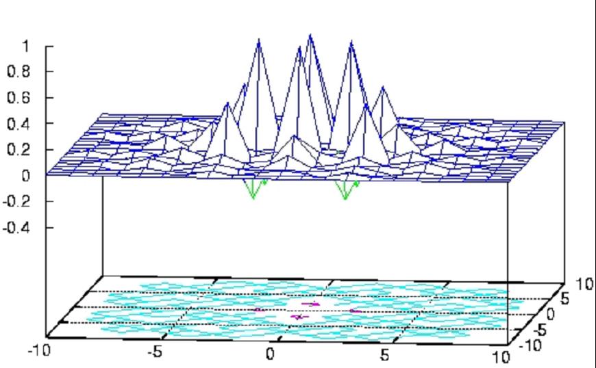
The exchange of the Fe sites is not limited to nearest neighbors and
can be ferromagnetic (positive) or antiferromagnetic (negative) (see
Fig. 2.4). Based on those facts and
the ab-initio
calculated parameters, the authors of Ref. [Mryasov 05]
introduced an effective hamiltonian that includes only the Fe
magnetic moment degrees of freedom:
and `soft' Pt layers).
The exchange of the Fe sites is not limited to nearest neighbors and
can be ferromagnetic (positive) or antiferromagnetic (negative) (see
Fig. 2.4). Based on those facts and
the ab-initio
calculated parameters, the authors of Ref. [Mryasov 05]
introduced an effective hamiltonian that includes only the Fe
magnetic moment degrees of freedom:
|
|